Jupyter Notebooks for Development

Jupyter notebooks are a useful tool for quick prototyping, live demonstrations of running code, and even a high-level software development. They are an interactive Python tool that can visualize data structures, run small snippets of code independently, and create complete workflows.

Jupyter notebooks have applications in data science, such as data visualization. However, they can be beneficial in network automation development to promote modular coding, good documentation, and quick demos and experiments. Finally, Jupyter Notebooks are a great tool for Python beginners. The benefits of using these notebooks are:

• Interactive prompts that can assist in finding errors and get quick feedback on how the code works,
• Visualization variables, data structures, and graphs,
• Unlike other interactive interpreters such as ipython where the script cannot be saved, these notebooks give you the ability to save and rerun,
• Integration of code with Markdown documentation,
• Small code blocks that lead to modular design.

In this blog, you will review how to set up your Visual Studio (VS) Code environment for Jupyter notebooks and use Poetry for package management. You will find several examples that demonstrate the power of developing Python scripts with Jupyter notebooks. By the end of this reading, you will be able to work with Jupyter notebooks for quick prototyping or extensive Python development.

You will find all examples referenced below in the Jupyter Blog GitHub repository.

Jupyter VS Code extension

ms-toolsai.jupyter

VS Code has an extension for Jupyter notebooks that you can easily install. You may add it from the extensions GUI, by using the extension reference that is linked above, or after creating a file with the extension ipynb you will be prompted to install it.

Using Poetry with Jupyter Notebooks

Package management can be tricky in Python projects and even more when using Jupyter notebooks, where a Python kernel needs to be defined in each one of them. We will use Poetry for managing dependencies. Poetry is an efficient dependency management tool set that supports package management and virtual environments. Below, we will set up our initial repository and environment for Jupyter notebook development, assuming that you have installed the Jupyter VS code extension.

First, create a new repository and initialize it using the following command:

> poetry init

This command will guide you through creating your pyproject.toml config.

Package name [jupyter-blog]:  
Version [0.1.0]:  
Description []:  Code for jupyter blog
Author [DrX <xenia.mountrouidou@networktocode.com>, n to skip]:  drx
License []:  
Compatible Python versions [^3.8]:  

Would you like to define your main dependencies interactively? (yes/no) [yes] no
Would you like to define your development dependencies interactively? (yes/no) [yes] no
Generated file

[tool.poetry]
name = "jupyter-blog"
version = "0.1.0"
description = "Code for jupyter blog"
authors = ["drx"]

[tool.poetry.dependencies]
python = "^3.8"

[tool.poetry.dev-dependencies]

[build-system]
requires = ["poetry-core>=1.0.0"]
build-backend = "poetry.core.masonry.api"


Do you confirm generation? (yes/no) [yes] 

Then, add Jupyter in the packages managed by poetry:

> poetry add jupyter

NOTE

You may add any other dependencies, like pandas, numpy, requests, etc. We will keep this minimal for now, since we mainly want to set up the Jupyter notebook with the Poetry virtual environment.

Linking Your Virtual Environment to Jupyter Kernel

When you first open your Jupyter notebook, it will pick the default Python environment, not your virtual environment that is managed by Poetry:

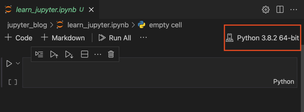
Below, you will find two methods to link the virtual environment to your kernel:

Using .vscode Settings

Notice that VS code creates a .vscode directory with local settings for this specific repo. Run the commands:

poetry shell
which python
/home/drx/.cache/pypoetry/virtualenvs/jupyter-blog-DRQV1zua-py3.8/bin/python

The first command will get you in the virtual environment you just created where Jupyter and your repo code are installed. The second command will give you the exact path that you need to use in your local repo settings. The name jupyter-blog-DRQV1zua-py3.8 is given by poetry to the virtual environment and it is based on the name of the repo, a hash, and the Python version. Copy and paste the Python path to the file .vscode/settings.json:

{
	"python.pythonPath": "/home/drx/.cache/pypoetry/virtualenvs/pandas-blog-vhxeqrbo-py3.8/bin/python",
}

You may need to restart VS Code for these changes to take effect.

Using symlink

Another method to link your virtual environment is with a symlink. The following command will create a link between your Poetry virtual environment and VS Code:

ln -s $(poetry env info -p) .venv

In this case, you will not need to restart VS Code, and you will quickly have a link of your Jupyter notebook kernel to the Python virtual environment managed by Poetry.

NOTE

Add the .venv and .vscode to your .gitignore to keep your repository clean from these environment-specific files.

The end result of both the above methods is a link between all your notebooks in this specific repository and the Poetry virtual environment. Furthermore, all the packages that you will add in this virtual environment from now on will be automatically included with your Jupyter kernel.

Features

You will now review the features of Jupyter notebooks that make it worth your time using them.

Cells

Cells are the killer feature of Jupyter Notebooks. They are structured as small snippets of code. A cell revolves around what you want to print or visualize. It is not a complete function or an object, although there are no hard rules that prevent you from adding a complete function in a cell. A rule of thumb when you are structuring your notebook is to think of your cells as opportunities to print and visualize.

We will add some interesting libraries to our environment to demonstrate the power of Jupyter notebooks:

poetry add pandas pytest matplotlib

Now we can create some cells:

import pandas as pd

# a pandas dataframe, i.e., a two-dimensional array
d = {'col1': [1, 2], 'col2': [3, 4]}

df = pd.DataFrame(data=d)
df.index = ['row1', 'row2']
df

Copy the above code in your cell, then hit the run button and you will get a nice visualization of what the dataframe looks like:

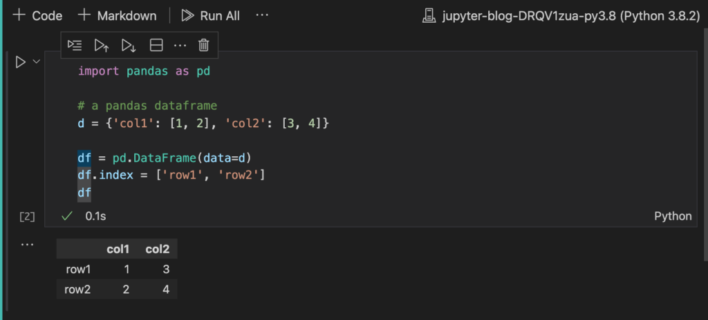
That last variable df prints the data frame without needing to use the print function. You will notice this pattern a lot in the cells.

Menus

There are two sets of menus: the ones that are on the notebook scope and the ones that are on cell scope. The notebook menus include the following functionality:

• Code: A standard code cell that has Python syntax highlighting, can include line numbers if you select “Show Notebook Line Numbers” and even debug breakpoints.
• Markdown: A markdown cell with all the syntactic features for documentation.
• Run all: This option runs all cells. There are also options to run on cell only or all cells before or after the specific cell, as shown in the additional code cell menus below.
• Clear Outputs of All Cells: You can clear all the outputs, however this option does not restart the kernel, i.e., the numbered cells will keep increasing, indicating new commands and not a complete reset of the notebook.
• Restart: This is the option you want to use to restart the kernel and start the cell numbering from 1.
• Export: You may export your notebook to Python, HTML, and even a PDF.

The cell menus differ for Markdown—you mainly have the options to edit and view. For Code cells, you have additional options such as run all cells before / after this cell, and run just this cell.

Variables

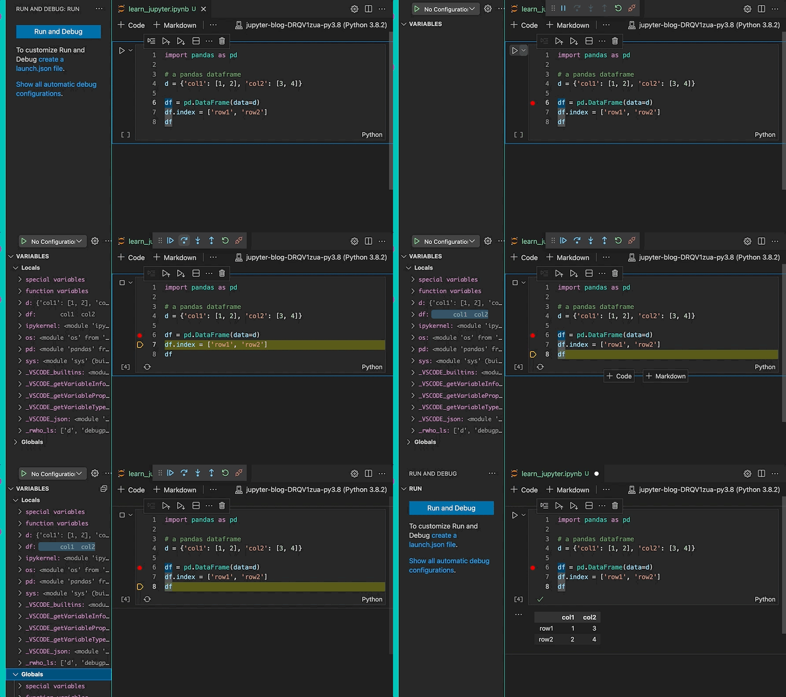
One of the less-appreciated features are the variables that can be used during runtime. The variables window shows the type, value, and size of a data structure. An example based on the code that you pasted above indicates that we have a dictionary and a DataFrame in our local variables. The size of the dictionary is 2, i.e., single dimension, and the DataFrame is a two-dimensional data structure with size (2, 2).

Debug

The last but not least feature is the debug. You can set breakpoints and observe the stack of execution as it builds with descriptive visualizations.

Applications

The next few examples demonstrate the power of Jupyter notebook applications.

Data structure visualization

One of the coolest ways to visualize a table or DataFrame is by using a Jupyter notebook. Reading a csv or Excel file has never been so easy and visual:

Graphs

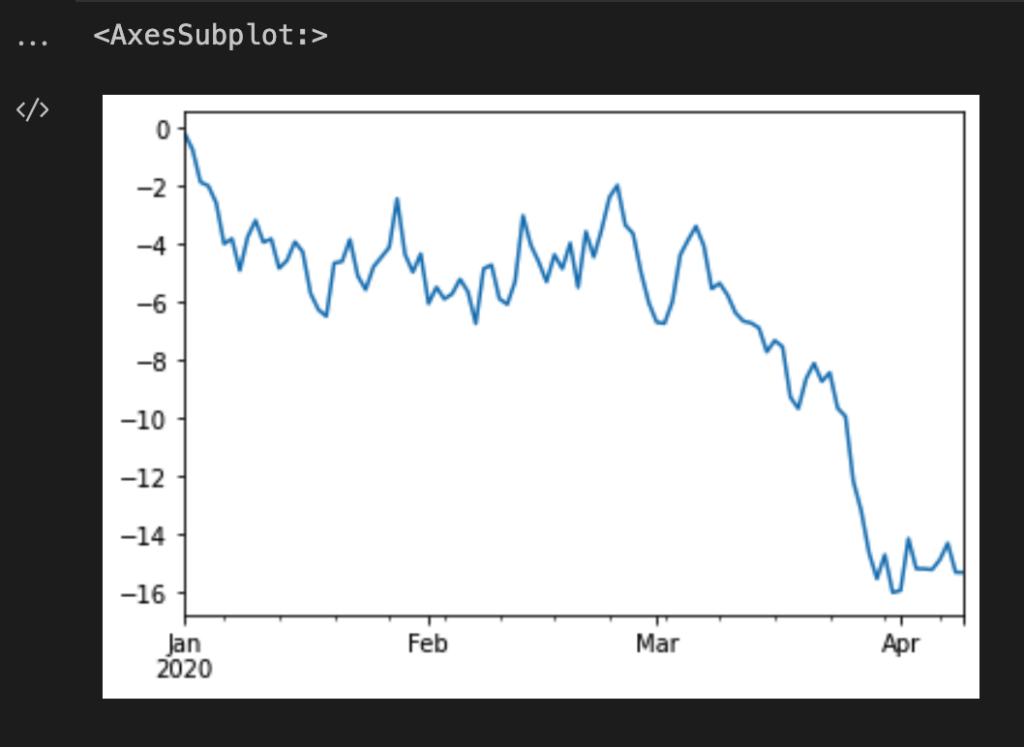
Another feature that your interactive Python interpreter does not include is visualizing graphs quickly and allowing for experimentation.

Time Series Graph

import numpy as np
import matplotlib

time_series = pd.Series(np.random.randn(100), index=pd.date_range("1/1/2020", periods=100))
time_series = time_series.cumsum()
time_series.plot()

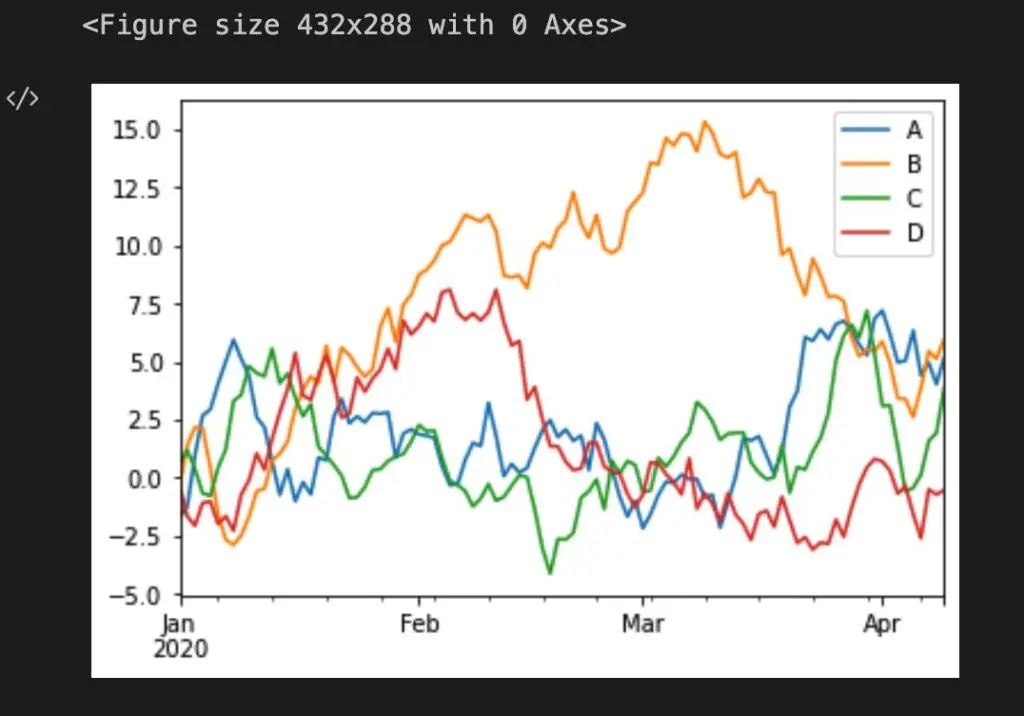
Dataframe graph

import matplotlib.pyplot as plt

df = pd.DataFrame(np.random.randn(100, 4), index=time_series.index, columns=list("ABCD"))
df = df.cumsum()
plt.figure()
df.plot()

Unit Testing

Unit testing can be performed seamlessly with a Jupyter notebook. The assertions can run in a cell and generate errors quickly every time you add new code.

A simple function that is validating router names is listed below:

import re

def validate_rtr_name(name):
    if re.match('[A-Z]{2}-rtr-\d{3}', name):
        return True
    else:
        return False

There are several unit tests listed below that can run in one cell:

assert validate_rtr_name('IL-rtr-421') == True

assert validate_rtr_name('ILQ-rtr-421') == False

assert validate_rtr_name('SC-rtr-41') == False

assert validate_rtr_name('SCrtr-41') == True

assert validate_rtr_name('SC-41') == False