Introduction to a Telemetry Stack – Part 2

Blog Detail

Just like The Fast and the Furious movies, we are going to be churning out sequels like no other! Welcome to Part 2 of the Telemetry Stack! series, where we walk you through the different stages of bringing insight into your infrastructure. Although there won’t be a special appearance from Ludacris in this sequel, you are in for a heck of a ride!

In this post we will focus on the concept of normalizing data between multiple systems and adding value with enrichment. To help follow along with some of the keywords used in this post, I recommend checking out Part 1 written by Nikos Kallergis for a refresher.

Normalization and Enrichment

During Part 1 we discussed the TPG stack, its different layers, and how to get started with Telegraf. Now it’s time to talk about processing those metrics into something more useful!

Have you ever run into the issue where different versions of software return different metric names like bgp_neighbor versus bgp-neighbor? What about metrics that don’t quite have all the data you’d like? This is where processing can help solve a lot of headaches by allowing you to normalize and enrich the metrics before passing them into your database.

Normalizing Data

One of the toughest situations to work with in telemetry is that almost every vendor is different. This means that sometimes your BGP metrics can come in with different labels or fields, which can introduce all kinds of trouble when trying to sort them in graphs or alerting. Normalizing the data allows you to adjust different fields and labels to either tune them to your environment, or to enforce naming standards.

Enriching Data

Enriching data can be very powerful and can take your metrics to a whole new level. Sure, some vendors do an amazing job at returning all the data you need, but what about the data that they can’t provide? With data enrichment you can add labels or fields to your metrics to track things like site location, rack location, customer IDs, and even SLA information for tenants.

NOTE:
Prometheus uses labels to determine the uniqueness of a metric. If you change the label of an existing metric, you may lose graph history in Grafana. You would need to update your query to pull for both the old and new labels so that they are combined.

Normalizing Data Using Telegraf

Using our scenario from above, let’s normalize some BGP data and modify a few metric fields to make sure they match and are standard across the board.

`[[processors.rename]]`

  # ---------------------------------------------------
  # Normalize BGP Data
  # ---------------------------------------------------
  [[processors.rename]]
    order = 1
    namepass = ["bgp*"]

    [[processors.rename.replace]]
      field = "installed"
      dest = "prefixes_installed"

    [[processors.rename.replace]]
      field = "sent"
      dest = "prefixes_sent"

    [[processors.rename.replace]]
      field = "received"
      dest = "prefixes_received"

It looks like a bit of a mess at first; but if you look closely, it’s pretty straightforward. [[processors.rename]]

order allows us to set the order in which processors are executed. It’s not required; but if you don’t specify, the order will be random.
namepass is an array of glob pattern strings. Only measurements’ names that match this pattern will be emitted.

With a simple processor like this, we are able to catch any BGP fields that come in as installed and transform them into prefixes_installed to ensure they match our metrics pulled from other agents.

- bgp_neighbor{installed="100", sent="100", received="150", neighbor="10.17.17.1"} 1
+ bgp_neighbor{prefixes_installed="100", prefixes_sent="100", prefixes_received="150", neighbor="10.17.17.1"} 1

`[[processors.enum]]`

Another powerful processor in Telegraf is enum. The enum processor allows the configuration of value mappings for field or tag values. The main use for this is for creating a mapping between strings and integers.

  # ---------------------------------------------------
  # Normalize status codes
  # ---------------------------------------------------
  [[processors.enum]]
    order = 3
    namepass = ["storage"]

    [[processors.enum.mapping]]
      tag = "status"
      [processors.enum.mapping.value_mappings]
        1 = "READ_ONLY"
        2 = "RUN_FROM_FLASH"
        3 = "READ_WRITE"

With this enum config, all storage metrics will have their status tag updated so that the end result is no longer a number and is easier to read.

- storage{type="scsi", status="1", host="server01"} 1500000
+ storage{type="scsi", status="READ_ONLY", host="server01"} 1500000

Sometimes even simple normalizations can save you from some of those dreaded late-night calls from your NOC. Changing a field into a more user-friendly field will prevent a lot of headaches during outages as well.

Enriching Data Using Telegraf

When it comes to enrichment you can either perform a what we call a static enrichment or a dynamic enrichment. Static enrichment is based on the Telegraf configuration file which means it is valid during the lifecycle of the configuration. Sometimes we like flexibility and not have a dependency on configuration or Telegraf deployments which is where dynamic enrichment comes in.

Static Enrichment

Telegraf has a lot of processors for enrichment but we will focus on the regex plugin. This plugin allows you to match a particular pattern for creating static labels and values.

  [[processors.regex]]
    order = 3
    namepass = ["interface_admin_status"]

    [processors.regex.tagpass]
      device = ["ceos-01"]

    [[processors.regex.tags]]
        key = "interface"
        pattern = "^Management1$"
        replacement = "mgmt"
        result_key = "intf_role"

- interface_admin_status{device="ceos-01", interface="Management1"} 1
+ interface_admin_status{device="ceos-01", interface="Management1", intf_role="mgmt"} 1

This is great, but wouldn’t it be better if this label could be updated with a change inside Nautobot? Well, this is where dynamic enrichment comes in.

Dynamic Enrichment

With dynamic enrichment we can take it a step further by pulling values from a single source of truth like Nautobot. In the next example I will be giving you a glance into an upcoming project that’s still currently in work but hopefully will be released soon so keep a lookout for the blog post!

Let me give you a sneak peek into network-agent. The network-agent project is built as a ‘batteries included’ Telegraf/Python-based container targeted for network metrics consumption and processing. The network-agent container comes with a lot of features, but for now we will only focus on the Nautobot processor.

Key features of this processor:

GraphQL-based queries to Nautobot for simplicity and speed.
JMESPath query for easy data extraction.
LRU caching to reduce API calls for metric enrichment.

NOTE:
The default cache TTL is set to 120 seconds. This means that the cache will remain valid until this timer has passed. After that, another GraphQL query to Nautobot is sent to check for new interfaces and roles.

This is what the configuration can look like:

[nautobot]
# Nautobot URL and Token specified using environment variables
graphql_query = """
query ($device: [String!]) {
  devices(name: $device) {
    name
    interfaces(tag: "intf_pri__tier1") {
      name
      cf_role
      tags {
        name
      }
    }
  }
}
"""

[enrich.interface.tag_pass]
  device = 'ceos-*'
  name = "interface*"

[enrich.interface.extract]  # JMESPATH
  interface_role = "devices[0].interfaces[?name==''].cf_role | [0]"

With this processor, we are able to query Nautobot for devices and filter the results to only interfaces with a intf_pri__tier1 tag. The information is then cached and can be used during the enrichment process.

`[enrich.interface.tag_pass]`

With the device and name options, we are able to control which specific metrics will get enriched with our new label.

`[enrich.interface.extract]`

This is where we define our new label that will get added to the metrics and the JMESPath query to grab our value. In this case, we will be taking the custom field called role out of Nautobot and adding it to all our interface metrics for our ceos devices.

- interface_admin_status{device="ceos-01", interface="Ethernet1"} 1
+ interface_admin_status{device="ceos-01", interface="Ethernet1", interface_role="border"} 1

Conclusion

Metric labels can be extremely powerful for both troubleshooting global infrastructure and capacity planning for companies. Whether you are using enrichment to add customer_id to BGP metrics or using normalization to remove those pesky special characters from your interface descriptions, telemetry can do it all.

-Donnie

Tags :

gnmi monitoring networking snmp telegraf telemetry telemetry-stack tutorial

Does this all sound amazing? Want to know more about how Network to Code can help you do this, reach out to our sales team. If you want to help make this a reality for our clients, check out our careers page.

Contact Us to Learn More

Share details about yourself & someone from our team will reach out to you ASAP!

Introduction to a Telemetry Stack – Part 1

Blog Detail

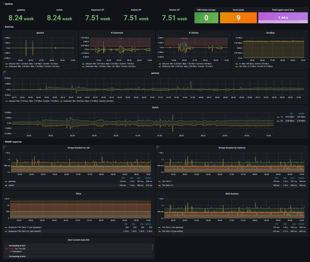
You know that “bookending” technique in movies like Fight Club and Pulp Fiction where they open up with the chronologically last scene? Well, this is more or less the same, but instead of a movie it’s the Telemetry Stack! NTC blog post series. And this is what your network monitoring solution could look like. Well, maybe not exactly like this but you get the idea, right?

This series of blog posts that will be released during the coming weeks dives into detail on how to build a contemporary network monitoring system using widely accepted open-source materials like Telegraf, Prometheus, Grafana, and Nautobot. Also, lots of “thanks” go to Josh VanDeraa and his very detailed blog posts that have served as a huge inspiration for this series!

In part 1 of the series, we’ll focus on two aspects:

Introduction to the Telemetry Stack!
Capturing metrics and data using Telegraf

Introduction to the Telemetry Stack!

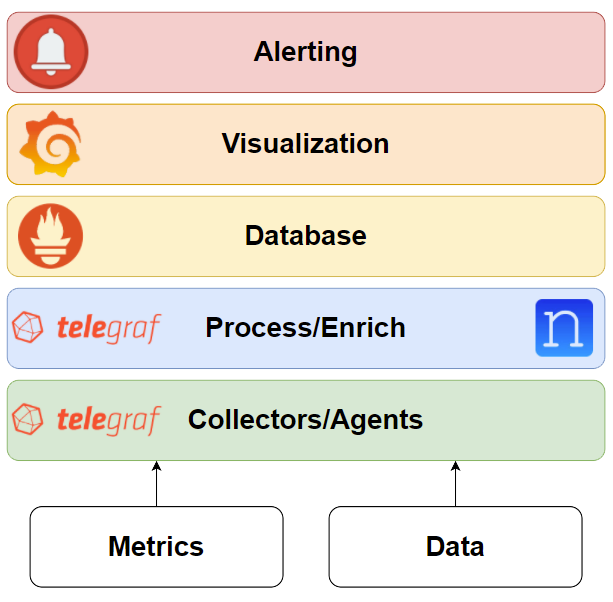
During the blog post series, we’ll explore the components that comprise the TPG (Telegraf, Prometheus, Grafana) Telemetry Stack!

Telegraf

In short, Telegraf is a metrics and events collector written in Go. Its simple architecture and plethora of built-in modules allow for easy capturing of metrics (input modules), linear processing (processor modules), and storing them to a multitude of back-end systems (output modules). For the enrichment part, Nautobot will be leveraged as the Source of Truth (SoT) that holds the additional information.

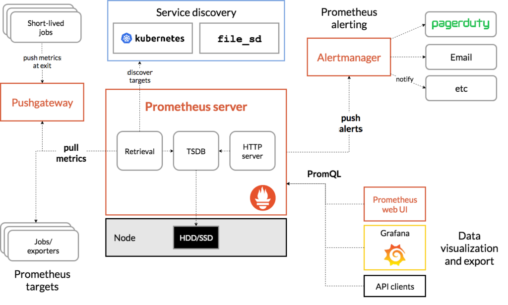
Prometheus

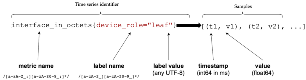
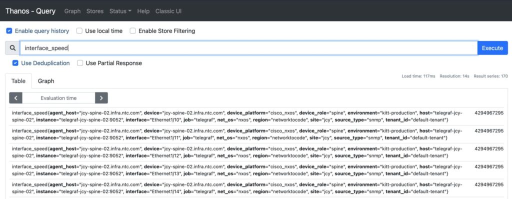
As already mentioned, Prometheus will be the TSDB of choice for storing our processed metrics and data.

Grafana

In order to present the data in a human-friendly form, we’ll be visualizing them using Grafana. Dashboard design is an art of its own, but we’ll attempt to present a basic set of dashboards that could serve as inspiration for creating your own.

Alertmanager

Using Grafana dashboards sprinkled with sane thresholds, we’re able to create alerting mechanisms triggered whenever a threshold is crossed.

Capturing Metrics and Data Using Telegraf

The rest of this post is dedicated on using Telegraf to get data from network devices. Now, one (or probably more) may wonder “why Telegraf?” and that’s indeed a question we also asked ourselves when designing this series. We decided to go with Telegraf based on the following factors:

it works and we like it
its configuration is comparatively easy to generate using templates
it’s a very flexible solution, allowing us to do SNMP, gNMI, and also execute Python scripts
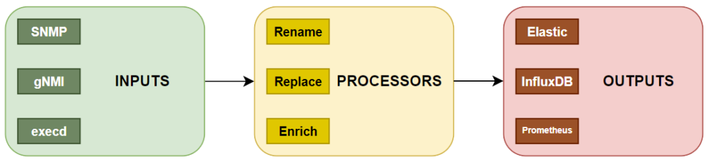
it uses a very simple basic flow between its components

Inputs: Telegraf provides a ton of various input methods out of the box, like snmp, gnmi, and execd. These are the components that enable us to capture metrics and data from our targets. Incidentally, this is also the main topic in the second half of this post, so more details may be found there.

Processors: As with inputs, Telegraf also comes loaded with a bunch of processor modules that allow us to manipulate our collected data. In this blog post series, our focus will be normalization and enrichment of the captured metrics. This will be the main topic in the second post of the series.

Outputs: Last, once we’re happy with the processors result, we use outputs to store the transformed data. Three of the most common Time Series Databases (TSDBs), used for storing metrics are InfluxDB (from the same manufacturer as Telegraf), Elasticsearch, and of course Prometheus which will be the output used throughout the series.

For the purposes of this blog post, we’ll be using two Arista cEOS machines. So, with all that out of our way, let’s dive into our various input methods!

`[[inputs.snmp]]`

Like the old-time gray-beards that we are, we’ll begin our journey using SNMP to perform a simple metrics capture.

# ------------------------------------------------
# Input - SNMP
# ------------------------------------------------
[[inputs.snmp]]
  agents = ["ceos-02"]
  version = 2
  community = "${SNMPv2_COMMUNITY}"
  interval = "60s"
  timeout = "10s"
  retries = 3

  [inputs.snmp.tags]
    collection_method = "snmp"
    device = "ceos-02"
    device_role = "router"
    device_platform = "arista"
    site = "lab-site-01"
    region = "lab"
    net_os = "eos"
  # ------------------------------------------------
  # Device Uptime (SNMP)
  # ------------------------------------------------
  [[inputs.snmp.field]]
    name = "uptime"
    oid = "RFC1213-MIB::sysUpTime.0"

  # ----------------------------------------------
  # Device Storage Partition Table polling (SNMP)
  # ----------------------------------------------
  [[inputs.snmp.table]]
    name = "storage"

    # Partition name
    [[inputs.snmp.table.field]]
      name = "name"
      oid = "HOST-RESOURCES-MIB::hrStorageDescr"
      is_tag = true

    # Size in bytes of the data objects allocated to the partition
    [[inputs.snmp.table.field]]
      name = "allocation_units"
      oid = "HOST-RESOURCES-MIB::hrStorageAllocationUnits"

    # Size of the partition storage represented by the allocation units
    [[inputs.snmp.table.field]]
      name = "size_allocation_units"
      oid = "HOST-RESOURCES-MIB::hrStorageSize"

    # Amount of space used by the partition represented by the allocation units
    [[inputs.snmp.table.field]]
      name = "used_allocation_units"
      oid = "HOST-RESOURCES-MIB::hrStorageUsed"

Note: A detailed line-by-line explanation of the Telegraf configuration may be found in the excellent Network Telemetry for SNMP Devices blog post by Josh.

`[[inputs.gnmi]]`

Now that we’ve covered the capabilities of old-school MIB/OID-based NMS, let’s jump to what all the cool kids are playing with these days: gRPC (Remote Procedure Calls) Network Management Interface. Bit of a mouthful! The main benefits of using gNMI for telemetry are its speed and efficiency. Thanks to the magic of Telegraf, we are able to capture data with just a few more lines of code.

# ------------------------------------------------
# Input - gNMI
# ------------------------------------------------
[[inputs.gnmi]]
  addresses = ["ceos-02:50051"]
  username = "${NETWORK_AGENT_USER}"
  password = "${NETWORK_AGENT_PASSWORD}"
  redial = "20s"
  tagexclude = [
      "identifier",
      "network_instances_network_instance_protocols_protocol_name",
      "afi_safi_name",
      "path",
      "source"
  ]

  [inputs.gnmi.tags]
    collection_method = "gnmi"
    device = "ceos-02"
    device_role = "router"
    device_platform = "arista"
    site = "lab-site-01"
    region = "lab"
    net_os = "eos"

  # ---------------------------------------------------
  # Device Interface Counters (gNMI)
  # ---------------------------------------------------
  [[inputs.gnmi.subscription]]
    name = "interface"
    path = "/interfaces/interface/state/counters"
    subscription_mode = "sample"
    sample_interval = "10s"

  [[inputs.gnmi.subscription]]
    name = "interface"
    path = "/interfaces/interface/state/admin-status"
    subscription_mode = "sample"
    sample_interval = "10s"

  [[inputs.gnmi.subscription]]
    name = "interface"
    path = "/interfaces/interface/state/oper-status"
    subscription_mode = "sample"
    sample_interval = "10s"

  # ---------------------------------------------------
  # Device Interface Ethernet Counters (gNMI)
  # ---------------------------------------------------
  [[inputs.gnmi.subscription]]
    name = "interface"
    path = "/interfaces/interface/ethernet/state/counters"
    subscription_mode = "sample"
    sample_interval = "10s"

  # ----------------------------------------------
  # Device CPU polling (gNMI)
  # ----------------------------------------------
  [[inputs.gnmi.subscription]]
    name = "cpu"
    path = "/components/component/cpu/utilization/state/instant"
    subscription_mode = "sample"
    sample_interval = "10s"

  # ----------------------------------------------
  # Device Memory polling (gNMI)
  # ----------------------------------------------
  [[inputs.gnmi.subscription]]
    name = "memory"
    path = "/components/component/state/memory"
    subscription_mode = "sample"
    sample_interval = "10s"

Note: Another great blog from Josh touches on the same subjects: Monitor Your Network With gNMI, SNMP, and Grafana.

`[[inputs.execd]]`

The third and last input that we’ll examine in this blog is execd; even cooler than the gNMI cool kids! Practically, it’s a way for Telegraf to run scripts and capture the data that are output in a metrics format. In our case though, the script is in reality a container image that makes it easy to collect metrics using a multitude of different methods. In the following simple example, it is used to collect BGP information over EOS RESTful API.

# ------------------------------------------------
# Input - Execd command
# ------------------------------------------------
[[inputs.execd]]
  interval = "60s"
  signal = "SIGHUP"
  restart_delay = "10s"
  data_format = "influx"
  command = [
    '/usr/local/bin/network_agent',
    '-h',
    'ceos-02',
    '-d',
    'arista_eos',
    '-c',
    'bgp_sessions::http',  ]
  [inputs.execd.tags]
    collection_method = "execd"
    device = "ceos-02"
    device_role = "router"
    device_platform = "arista"
    site = "lab-site-01"
    region = "lab"
    net_os = "eos"

Collected Data

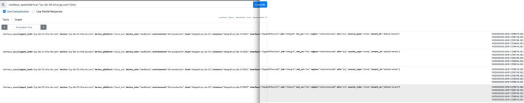
At this point, we’ve managed to collect various metrics and data from our target devices. We still have to process them, store them, and visualize them but these are the topics of the blog posts that will follow. For now, we may take a peek into the collected data to verify that they’ve been captured successfully, before “passing” them to the normalization/enrichment step of the process.

`[[inputs.snmp]]`

# HELP snmp_uptime Telegraf collected metric
# TYPE snmp_uptime untyped
snmp_uptime{collection_method="snmp",device="ceos-01",device_platform="arista",device_role="router",environment="dev",host="telegraf-01",net_os="eos",region="lab",site="lab-site-01"} 14082

# HELP storage_allocation_units Telegraf collected metric
# TYPE storage_allocation_units untyped
storage_allocation_units{collection_method="snmp",device="ceos-01",device_platform="arista",device_role="router",environment="dev",host="telegraf-01",name="Core",net_os="eos",region="lab",site="lab-site-01"} 4096
storage_allocation_units{collection_method="snmp",device="ceos-01",device_platform="arista",device_role="router",environment="dev",host="telegraf-01",name="Flash",net_os="eos",region="lab",site="lab-site-01"} 4096
storage_allocation_units{collection_method="snmp",device="ceos-01",device_platform="arista",device_role="router",environment="dev",host="telegraf-01",name="Log",net_os="eos",region="lab",site="lab-site-01"} 4096
storage_allocation_units{collection_method="snmp",device="ceos-01",device_platform="arista",device_role="router",environment="dev",host="telegraf-01",name="RAM",net_os="eos",region="lab",site="lab-site-01"} 1024
storage_allocation_units{collection_method="snmp",device="ceos-01",device_platform="arista",device_role="router",environment="dev",host="telegraf-01",name="RAM (Buffers)",net_os="eos",region="lab",site="lab-site-01"} 1024
storage_allocation_units{collection_method="snmp",device="ceos-01",device_platform="arista",device_role="router",environment="dev",host="telegraf-01",name="RAM (Cache)",net_os="eos",region="lab",site="lab-site-01"} 1024
storage_allocation_units{collection_method="snmp",device="ceos-01",device_platform="arista",device_role="router",environment="dev",host="telegraf-01",name="RAM (Unavailable)",net_os="eos",region="lab",site="lab-site-01"} 1024
storage_allocation_units{collection_method="snmp",device="ceos-01",device_platform="arista",device_role="router",environment="dev",host="telegraf-01",name="Root",net_os="eos",region="lab",site="lab-site-01"} 4096
storage_allocation_units{collection_method="snmp",device="ceos-01",device_platform="arista",device_role="router",environment="dev",host="telegraf-01",name="Tmp",net_os="eos",region="lab",site="lab-site-01"} 4096
# HELP storage_size_allocation_units Telegraf collected metric
# TYPE storage_size_allocation_units untyped
storage_size_allocation_units{collection_method="snmp",device="ceos-01",device_platform="arista",device_role="router",environment="dev",host="telegraf-01",name="Core",net_os="eos",region="lab",site="lab-site-01"} 400150
storage_size_allocation_units{collection_method="snmp",device="ceos-01",device_platform="arista",device_role="router",environment="dev",host="telegraf-01",name="Flash",net_os="eos",region="lab",site="lab-site-01"} 2.5585863e+07
storage_size_allocation_units{collection_method="snmp",device="ceos-01",device_platform="arista",device_role="router",environment="dev",host="telegraf-01",name="Log",net_os="eos",region="lab",site="lab-site-01"} 400150
storage_size_allocation_units{collection_method="snmp",device="ceos-01",device_platform="arista",device_role="router",environment="dev",host="telegraf-01",name="RAM",net_os="eos",region="lab",site="lab-site-01"} 1.6005976e+07
storage_size_allocation_units{collection_method="snmp",device="ceos-01",device_platform="arista",device_role="router",environment="dev",host="telegraf-01",name="RAM (Buffers)",net_os="eos",region="lab",site="lab-site-01"} 1.6005976e+07
storage_size_allocation_units{collection_method="snmp",device="ceos-01",device_platform="arista",device_role="router",environment="dev",host="telegraf-01",name="RAM (Cache)",net_os="eos",region="lab",site="lab-site-01"} 1.6005976e+07
storage_size_allocation_units{collection_method="snmp",device="ceos-01",device_platform="arista",device_role="router",environment="dev",host="telegraf-01",name="RAM (Unavailable)",net_os="eos",region="lab",site="lab-site-01"} 1.6005976e+07
storage_size_allocation_units{collection_method="snmp",device="ceos-01",device_platform="arista",device_role="router",environment="dev",host="telegraf-01",name="Root",net_os="eos",region="lab",site="lab-site-01"} 2.5585863e+07
storage_size_allocation_units{collection_method="snmp",device="ceos-01",device_platform="arista",device_role="router",environment="dev",host="telegraf-01",name="Tmp",net_os="eos",region="lab",site="lab-site-01"} 16384
# HELP storage_used_allocation_units Telegraf collected metric
# TYPE storage_used_allocation_units untyped
storage_used_allocation_units{collection_method="snmp",device="ceos-01",device_platform="arista",device_role="router",environment="dev",host="telegraf-01",name="Core",net_os="eos",region="lab",site="lab-site-01"} 0
storage_used_allocation_units{collection_method="snmp",device="ceos-01",device_platform="arista",device_role="router",environment="dev",host="telegraf-01",name="Flash",net_os="eos",region="lab",site="lab-site-01"} 7.955702e+06
storage_used_allocation_units{collection_method="snmp",device="ceos-01",device_platform="arista",device_role="router",environment="dev",host="telegraf-01",name="Log",net_os="eos",region="lab",site="lab-site-01"} 14989
storage_used_allocation_units{collection_method="snmp",device="ceos-01",device_platform="arista",device_role="router",environment="dev",host="telegraf-01",name="RAM",net_os="eos",region="lab",site="lab-site-01"} 7.242028e+06
storage_used_allocation_units{collection_method="snmp",device="ceos-01",device_platform="arista",device_role="router",environment="dev",host="telegraf-01",name="RAM (Buffers)",net_os="eos",region="lab",site="lab-site-01"} 953836
storage_used_allocation_units{collection_method="snmp",device="ceos-01",device_platform="arista",device_role="router",environment="dev",host="telegraf-01",name="RAM (Cache)",net_os="eos",region="lab",site="lab-site-01"} 2.134188e+06
storage_used_allocation_units{collection_method="snmp",device="ceos-01",device_platform="arista",device_role="router",environment="dev",host="telegraf-01",name="RAM (Unavailable)",net_os="eos",region="lab",site="lab-site-01"} 4.148248e+06
storage_used_allocation_units{collection_method="snmp",device="ceos-01",device_platform="arista",device_role="router",environment="dev",host="telegraf-01",name="Root",net_os="eos",region="lab",site="lab-site-01"} 7.955702e+06
storage_used_allocation_units{collection_method="snmp",device="ceos-01",device_platform="arista",device_role="router",environment="dev",host="telegraf-01",name="Tmp",net_os="eos",region="lab",site="lab-site-01"} 0

`[[inputs.gnmi]]`

# HELP cpu_instant Telegraf collected metric
# TYPE cpu_instant untyped
cpu_instant{collection_method="gnmi",device="ceos-01",device_platform="arista",device_role="router",environment="dev",host="telegraf-01",name="CPU0",net_os="eos",region="lab",site="lab-site-01"} 3
cpu_instant{collection_method="gnmi",device="ceos-01",device_platform="arista",device_role="router",environment="dev",host="telegraf-01",name="CPU1",net_os="eos",region="lab",site="lab-site-01"} 5
cpu_instant{collection_method="gnmi",device="ceos-01",device_platform="arista",device_role="router",environment="dev",host="telegraf-01",name="CPU2",net_os="eos",region="lab",site="lab-site-01"} 3
cpu_instant{collection_method="gnmi",device="ceos-01",device_platform="arista",device_role="router",environment="dev",host="telegraf-01",name="CPU3",net_os="eos",region="lab",site="lab-site-01"} 3

# HELP interface_in_broadcast_pkts Telegraf collected metric
# TYPE interface_in_broadcast_pkts untyped
interface_in_broadcast_pkts{collection_method="gnmi",device="ceos-01",device_platform="arista",device_role="router",environment="dev",host="telegraf-01",name="Ethernet1",net_os="eos",region="lab",site="lab-site-01"} 0
# HELP interface_in_crc_errors Telegraf collected metric
# TYPE interface_in_crc_errors untyped
interface_in_crc_errors{collection_method="gnmi",device="ceos-01",device_platform="arista",device_role="router",environment="dev",host="telegraf-01",name="Ethernet1",net_os="eos",region="lab",site="lab-site-01"} 0
# HELP interface_in_discards Telegraf collected metric
# TYPE interface_in_discards untyped
interface_in_discards{collection_method="gnmi",device="ceos-01",device_platform="arista",device_role="router",environment="dev",host="telegraf-01",name="Ethernet1",net_os="eos",region="lab",site="lab-site-01"} 0
# HELP interface_in_errors Telegraf collected metric
# TYPE interface_in_errors untyped
interface_in_errors{collection_method="gnmi",device="ceos-01",device_platform="arista",device_role="router",environment="dev",host="telegraf-01",name="Ethernet1",net_os="eos",region="lab",site="lab-site-01"} 0
# HELP interface_in_fcs_errors Telegraf collected metric
# TYPE interface_in_fcs_errors untyped
interface_in_fcs_errors{collection_method="gnmi",device="ceos-01",device_platform="arista",device_role="router",environment="dev",host="telegraf-01",name="Ethernet1",net_os="eos",region="lab",site="lab-site-01"} 0
# HELP interface_in_fragment_frames Telegraf collected metric
# TYPE interface_in_fragment_frames untyped
interface_in_fragment_frames{collection_method="gnmi",device="ceos-01",device_platform="arista",device_role="router",environment="dev",host="telegraf-01",name="Ethernet1",net_os="eos",region="lab",site="lab-site-01"} 0
# HELP interface_in_jabber_frames Telegraf collected metric
# TYPE interface_in_jabber_frames untyped
interface_in_jabber_frames{collection_method="gnmi",device="ceos-01",device_platform="arista",device_role="router",environment="dev",host="telegraf-01",name="Ethernet1",net_os="eos",region="lab",site="lab-site-01"} 0
# HELP interface_in_mac_control_frames Telegraf collected metric
# TYPE interface_in_mac_control_frames untyped
interface_in_mac_control_frames{collection_method="gnmi",device="ceos-01",device_platform="arista",device_role="router",environment="dev",host="telegraf-01",name="Ethernet1",net_os="eos",region="lab",site="lab-site-01"} 0
# HELP interface_in_mac_pause_frames Telegraf collected metric
# TYPE interface_in_mac_pause_frames untyped
interface_in_mac_pause_frames{collection_method="gnmi",device="ceos-01",device_platform="arista",device_role="router",environment="dev",host="telegraf-01",name="Ethernet1",net_os="eos",region="lab",site="lab-site-01"} 0
# HELP interface_in_multicast_pkts Telegraf collected metric
# TYPE interface_in_multicast_pkts untyped
interface_in_multicast_pkts{collection_method="gnmi",device="ceos-01",device_platform="arista",device_role="router",environment="dev",host="telegraf-01",name="Ethernet1",net_os="eos",region="lab",site="lab-site-01"} 25
# HELP interface_in_octets Telegraf collected metric
# TYPE interface_in_octets untyped
interface_in_octets{collection_method="gnmi",device="ceos-01",device_platform="arista",device_role="router",environment="dev",host="telegraf-01",name="Ethernet1",net_os="eos",region="lab",site="lab-site-01"} 4349
# HELP interface_in_oversize_frames Telegraf collected metric
# TYPE interface_in_oversize_frames untyped
interface_in_oversize_frames{collection_method="gnmi",device="ceos-01",device_platform="arista",device_role="router",environment="dev",host="telegraf-01",name="Ethernet1",net_os="eos",region="lab",site="lab-site-01"} 0
# HELP interface_in_unicast_pkts Telegraf collected metric
# TYPE interface_in_unicast_pkts untyped
interface_in_unicast_pkts{collection_method="gnmi",device="ceos-01",device_platform="arista",device_role="router",environment="dev",host="telegraf-01",name="Ethernet1",net_os="eos",region="lab",site="lab-site-01"} 21
# HELP interface_out_broadcast_pkts Telegraf collected metric
# TYPE interface_out_broadcast_pkts untyped
interface_out_broadcast_pkts{collection_method="gnmi",device="ceos-01",device_platform="arista",device_role="router",environment="dev",host="telegraf-01",name="Ethernet1",net_os="eos",region="lab",site="lab-site-01"} 0
# HELP interface_out_discards Telegraf collected metric
# TYPE interface_out_discards untyped
interface_out_discards{collection_method="gnmi",device="ceos-01",device_platform="arista",device_role="router",environment="dev",host="telegraf-01",name="Ethernet1",net_os="eos",region="lab",site="lab-site-01"} 0
# HELP interface_out_errors Telegraf collected metric
# TYPE interface_out_errors untyped
interface_out_errors{collection_method="gnmi",device="ceos-01",device_platform="arista",device_role="router",environment="dev",host="telegraf-01",name="Ethernet1",net_os="eos",region="lab",site="lab-site-01"} 0
# HELP interface_out_mac_control_frames Telegraf collected metric
# TYPE interface_out_mac_control_frames untyped
interface_out_mac_control_frames{collection_method="gnmi",device="ceos-01",device_platform="arista",device_role="router",environment="dev",host="telegraf-01",name="Ethernet1",net_os="eos",region="lab",site="lab-site-01"} 0
# HELP interface_out_mac_pause_frames Telegraf collected metric
# TYPE interface_out_mac_pause_frames untyped
interface_out_mac_pause_frames{collection_method="gnmi",device="ceos-01",device_platform="arista",device_role="router",environment="dev",host="telegraf-01",name="Ethernet1",net_os="eos",region="lab",site="lab-site-01"} 0
# HELP interface_out_multicast_pkts Telegraf collected metric
# TYPE interface_out_multicast_pkts untyped
interface_out_multicast_pkts{collection_method="gnmi",device="ceos-01",device_platform="arista",device_role="router",environment="dev",host="telegraf-01",name="Ethernet1",net_os="eos",region="lab",site="lab-site-01"} 0
# HELP interface_out_octets Telegraf collected metric
# TYPE interface_out_octets untyped
interface_out_octets{collection_method="gnmi",device="ceos-01",device_platform="arista",device_role="router",environment="dev",host="telegraf-01",name="Ethernet1",net_os="eos",region="lab",site="lab-site-01"} 0
# HELP interface_out_unicast_pkts Telegraf collected metric
# TYPE interface_out_unicast_pkts untyped
interface_out_unicast_pkts{collection_method="gnmi",device="ceos-01",device_platform="arista",device_role="router",environment="dev",host="telegraf-01",name="Ethernet1",net_os="eos",region="lab",site="lab-site-01"} 0

# HELP memory_available Telegraf collected metric
# TYPE memory_available untyped
memory_available{collection_method="gnmi",device="ceos-01",device_platform="arista",device_role="router",environment="dev",host="telegraf-01",name="Chassis",net_os="eos",region="lab",site="lab-site-01"} 1.6390119424e+10
# HELP memory_utilized Telegraf collected metric
# TYPE memory_utilized untyped
memory_utilized{collection_method="gnmi",device="ceos-01",device_platform="arista",device_role="router",environment="dev",host="telegraf-01",name="Chassis",net_os="eos",region="lab",site="lab-site-01"} 7.414636544e+09

`[[inputs.execd]]`

# HELP bgp_sessions_prefixes_received Telegraf collected metric
# TYPE bgp_sessions_prefixes_received untyped
bgp_sessions_prefixes_received{collection_method="execd",device="ceos-01",device_platform="arista",device_role="router",environment="dev",host="telegraf-01",local_as="65111",neighbor_address="10.1.2.2",net_os="eos",peer_as="65222",peer_router_id="10.17.17.2",peer_type="external",region="lab",router_id="10.17.17.1",routing_instance="default",session_state="established",site="lab-site-01"} 1
bgp_sessions_prefixes_received{collection_method="execd",device="ceos-01",device_platform="arista",device_role="router",environment="dev",host="telegraf-01",local_as="65111",neighbor_address="10.1.7.2",net_os="eos",peer_as="65222",peer_router_id="0.0.0.0",peer_type="external",region="lab",router_id="10.17.17.1",routing_instance="default",session_state="active",site="lab-site-01"} 0
# HELP bgp_sessions_prefixes_sent Telegraf collected metric
# TYPE bgp_sessions_prefixes_sent untyped
bgp_sessions_prefixes_sent{collection_method="execd",device="ceos-01",device_platform="arista",device_role="router",environment="dev",host="telegraf-01",local_as="65111",neighbor_address="10.1.2.2",net_os="eos",peer_as="65222",peer_router_id="10.17.17.2",peer_type="external",region="lab",router_id="10.17.17.1",routing_instance="default",session_state="established",site="lab-site-01"} 1
bgp_sessions_prefixes_sent{collection_method="execd",device="ceos-01",device_platform="arista",device_role="router",environment="dev",host="telegraf-01",local_as="65111",neighbor_address="10.1.7.2",net_os="eos",peer_as="65222",peer_router_id="0.0.0.0",peer_type="external",region="lab",router_id="10.17.17.1",routing_instance="default",session_state="active",site="lab-site-01"} 0
# HELP bgp_sessions_session_state_code Telegraf collected metric
# TYPE bgp_sessions_session_state_code untyped
bgp_sessions_session_state_code{collection_method="execd",device="ceos-01",device_platform="arista",device_role="router",environment="dev",host="telegraf-01",local_as="65111",neighbor_address="10.1.2.2",net_os="eos",peer_as="65222",peer_router_id="10.17.17.2",peer_type="external",region="lab",router_id="10.17.17.1",routing_instance="default",session_state="established",site="lab-site-01"} 6
bgp_sessions_session_state_code{collection_method="execd",device="ceos-01",device_platform="arista",device_role="router",environment="dev",host="telegraf-01",local_as="65111",neighbor_address="10.1.7.2",net_os="eos",peer_as="65222",peer_router_id="0.0.0.0",peer_type="external",region="lab",router_id="10.17.17.1",routing_instance="default",session_state="active",site="lab-site-01"} 3

Conclusion

The best parts of the Telemetry Stack! series are yet to come, so stay tuned! For any question you may have, feel free to join our Slack community.

-Nikos

Tags :

gnmi monitoring networking snmp telegraf telemetry telemetry-stack tutorial

Contact Us to Learn More

Share details about yourself & someone from our team will reach out to you ASAP!

Introduction to PromQL

Blog Detail

Time series databases and their query languages are tools with increasing popularity for a Network Automation Engineer. However, sometimes these tools may be overlooked by network operators for more “pressing” day-to-day workflow automation. Time series databases offer valuable network telemetry that will reveal important insights for network operations, such as security breaches, network outages, and slowdowns that degrade the user experience.

In this post, we will review the Prometheus Query Language (PromQL) to demonstrate the value and capabilities of processing time series. This review will offer use cases of PromQL for network engineers and data scientists.

What is Prometheus?

Prometheus is an open source systems monitoring and alerting toolkit. As you can see in the figure below, the heart of Prometheus includes a Time Series Database (TSDB) and the PromQL Engine. Exporters run locally on monitored hosts and export local metrics related to device health, such as CPU and memory utilization, and services, such as HTTP. The alert mechanism implemented with Prometheus, triggers alerts based on events and predefined thresholds. Prometheus has a web UI that we will be using in the examples of this post. In addition, the Prometheus measurements can be visualized using Grafana dashboards.

Source: Prometheus Overview

What is a TSDB?

In simple words, it is a database that stores time series. Then, what is a time series? It is a set of time-stamps and their corresponding data. A TSDB is optimized to store these time series data efficiently, measure changes, and perform calculations over time. PromQL is the language that was built to retrieve data from the Prometheus TSDB. In networking, this could mean tracking the state of an interface or bandwidth utilization over time.

Why PromQL?

There are several other TSDBs, one of the most well known is InfluxDB. Both Prometheus TSDB and InfluxDB are excellent tools for telemetry and time series data manipulation. PromQL’s popularity has been growing fast because it is a comprehensive language to consume time series data. Multiple other solutions are starting to support PromQL, such as NewRelic that recently added support for PromQL and Timescale with Promscale.

Now that we have all the prerequisite knowledge we can dive deep into the PromQL data model and dissect language queries.

Prometheus Data Model

The first part of the Prometheus data model is the metric name. A metric name is uniquely identified, and it indicates what is being measured. A metric is a dimension of a specific feature. Labels are the second part of the data model. A label is a key-value pair that differentiates sub-dimensions in a metric.

Think of a metric, ex. interface_in_octets, as an object with multiple characteristics, ex., device_role. As you can see in the figure below, each label can pick a value for this characteristic, i.e. device_role="leaf". The combination of metrics and labels return a time series identifier, i.e., a list of tuples that provide the (timestamp, value) of the object with the specific characteristic. The timestamps are given in Unix time, milliseconds precision and the values that correspond to them are floating point type.

As a Network Automation Engineer you can think of many examples of metrics, such as interface_speed, bgp_hold_time, packets_dropped, etc. All these metrics can be characterized by a variety of labels, such as device_platform, host, instance, interface_name etc.

With that data model in mind, let us next dissect a query in PromQL.

The anatomy of a query

The simplest form of a PromQL query may include just a metric. This query returns multiple single value vectors, as you can see below. All the applicable labels and value combinations that these labels can be assigned are given as a result of this simple query.

Metrics

What kind of metrics does PromQL support? There are four kinds of metrics:

Counters: these are metrics that can only increase, for example: interface counters, API call counters, etc.
Gauges: the values of these metrics can go up and down, for example: bandwidth, latency, packets dropped, etc. Gauges and counters are useful for network engineers because they can measure already existent features of a system.
Summaries: this metric is useful to data scientists and if your application includes data analytics. To use this metric you need have control of what you can measure and drill into additional details. A summary metric aggregates thousands of events to one metric. Specifically it counts observations and sums all the observed values. It can also calculate quantiles of these values. If you have an application that is being monitored, you can use the summaries for API request durations.
Histograms: this is another metric that is more useful to a data scientist than a network engineer. Histogram metrics can be defined as summaries that are “bucketized”. Specifically they count observations and place them in configurable buckets. A histogram can be used to measure response sizes on an application.

Label Filtering

Now that we know what kinds of metrics we can include in our query, let us review how we can filter the query to retrieve more specific and meaningful results. This can be done with label filtering that includes the following operations:

# equal, returns interface speed for device with name jcy-bb-01
interface_speed{device="jcy-bb-01.infra.ntc.com"}
# not equal, returns the opposite of the above query
interface_speed{device!="jcy-bb-01.infra.ntc.com"}
# regex-match, matches interface Ethernet{1, 2, 3, 4, 5, 6, 7}
interface_speed{interface=~"Ethernet1/[1-7]"}
# not regex-match, returns the opposite of the above query
interface_speed{interface!~"Ethernet1/[1-7]"}

Not only can you use the equal and not equal signs to filter your queries, but you can filter using regular expressions. To learn more about regular expressions for network engineers, check our previous blog.

Functions

One of my favorite parts of PromQL are the functions that can manipulate the time series identifiers. Below, I include an example of the function rate(), that is useful for network metrics, and the function predict_linear(), that is useful if you perform data analytics.

How fast does a counter change?

The function rate() can be used with counter metrics to demonstrate how fast a counter increases. Specifically, it calculates the per second increase for a time period. This is a useful function to the network engineer, since counters are a common metric applied in networks. For example packet counting, interface octets counting are counters and the rate() function offers useful insights on how these counters increase.

#per second increase of counter averaged over 5 mins
rate(interface_in_octets{device_role="leaf"}[5m])

The next figure will help you understand the details of how the rate() function is calculated. The interval $\Delta$t indicates the time interval during which we want to calculate the rate. The X marks indicate the per second samples that are used to calculate multiple rates per second. The rate() function averages these calculations during the interval $\Delta$t. If the counter is reset to 0, the rate() function will extrapolate the sample as can be seen with the blue X marks.

Instance vs. Range Vectors

You probably have noticed that the example of the rate() function above, uses a different type of syntax. Specifically it identifies the time series during an interval, from the example above the interval is 5 minutes ([5m]). This results to a range vector, where the time-series identifier returns the values for a given period, in this case 5 minutes. On the other hand, an instance vector returns one value, specifically the single latest value of a time series. The figures below shows the differences in the results of an instance vector versus a range vector.

#instance vector
interface_speed{device="jcy-bb-01.infra.ntc.com"}

#range vector
interface_speed{device="jcy-bb-01.infra.ntc.com"}[5m]

In the first figure, only one value per vector is returned whereas in the second, multiple values that span in the range of 5 minutes are returned for each vector. The format of these values is: value@timestamp.

Offsets

You may be wondering: all of this is great, but where is the “time” in my “time-series”? The offset part of the query can retrieve data for a specific time interval. For example:

# interface speed status for the past 24 hrs
rate(interface_in_octets{device="jcy-bb-01.infra.ntc.com"}[5m] offset 24h)

Here we combine the function rate(), that samples the interface_in_octets counter every second for five minutes, with offset that gives us historical data for the past 24 hours.

Can I predict the next 24 hours?

Of course! PromQL provides the function predict_linear(), a simple machine learning model that predicts the value of a gauge in a given amount of time in the future, by using linear regression. This function is of more interest to a data scientist that wants to create forecasting models. For example, if you want to predict the disk usage in bytes within the next hour based on historic data, you would use the following query:

#predict disk usage bytes in an hour, using the last 15 mins of data
predict_linear(demo_disk_usage_bytes{job="demo"}[15m], 3600)

Linear regression fits a linear function to a set of random data points. This is achieved by searching for all possible values for the variables a, b that define a linear function f(x)=ax+b. The line that minimizes the mean Euclidean distance of all these data points is the result of the linear regression model, as you can see in the image below:

Aggregation

PromQL queries can be highly dimensional. This means that one query can return a set of time series identifiers for all the combinations of labels, as you can see below:

#multi-dimensional query
rate(demo_api_request_duration_seconds_count{job="demo"}[5m])

What if you want to reduce the dimensions to a more meaningful result, for example the sum of all the API request durations in seconds? This would result in a single-dimension query that is the result of adding multiple instance vectors together:

#one-dimensional query, add instance vectors
sum(rate(demo_api_request_duration_seconds_count{job="demo"}[5m]))

You may choose to aggregate over specific dimensions using labels and the function by(). In the example below, we perform a sum over all instances, paths, and jobs. Note the reduction of the number of vectors returned:

# multi-dimensional query - by()
sum by(instance, path, job) (rate(demo_api_request_duration_seconds_count{job="demo"}[5m]))

We can perform the same query excluding labels using the function without():

sum without(method, status) (rate(demo_api_request_duration_seconds_count{job="demo"}[5m]))

This results to the same set of instance vectors:

Additional aggregation over dimensions can be done with the following functions:

min(): selects the minimum of all values within an aggregated group.
max(): selects the maximum of all values within an aggregated group.
avg(): calculates the average (arithmetic mean) of all values within an aggregated group.
stddev(): calculates the standard deviation of all values within an aggregated group.
stdvar(): calculates the standard variance of all values within an aggregated group.
count(): calculates the total number of series within an aggregated group.
count_values(): calculates number of elements with the same sample value.

Useful Resources

PromQL Demo, official demo where you can practice PromQL queries.
Alerting with Prometheus blog by Josh VanDeraa, Network To Code.
Monitoring Websites with Telegraf and Prometheus blog by Josh VanDeraa, Network To Code.

Conclusion

Thank you for taking this journey with me, learning about the time series query language, PromQL. There are many more features to this language such as arithmetic, sorting, set functions etc. I hope that this post has given you the opportunity to understand the basics of PromQL, see the value of telemetry and TSDBs, and that it has increased your curiosity to learn more.

-Xenia

Tags :

automation monitoring netdevops prometheus telemetry tsdb tutorial

Contact Us to Learn More

Share details about yourself & someone from our team will reach out to you ASAP!

Cookie	Duration	Description
__hssc	30 minutes	HubSpot sets this cookie to keep track of sessions and to determine if HubSpot should increment the session number and timestamps in the __hstc cookie.
__hssrc	session	This cookie is set by Hubspot whenever it changes the session cookie. The __hssrc cookie set to 1 indicates that the user has restarted the browser, and if the cookie does not exist, it is assumed to be a new session.
cookielawinfo-checkbox-advertisement	1 year	Set by the GDPR Cookie Consent plugin, this cookie records the user consent for the cookies in the "Advertisement" category.
cookielawinfo-checkbox-analytics	11 months	This cookie is set by GDPR Cookie Consent plugin. The cookie is used to store the user consent for the cookies in the category "Analytics".
cookielawinfo-checkbox-functional	11 months	The cookie is set by GDPR cookie consent to record the user consent for the cookies in the category "Functional".
cookielawinfo-checkbox-necessary	11 months	This cookie is set by GDPR Cookie Consent plugin. The cookies is used to store the user consent for the cookies in the category "Necessary".
cookielawinfo-checkbox-others	11 months	This cookie is set by GDPR Cookie Consent plugin. The cookie is used to store the user consent for the cookies in the category "Other.
cookielawinfo-checkbox-performance	11 months	This cookie is set by GDPR Cookie Consent plugin. The cookie is used to store the user consent for the cookies in the category "Performance".
CookieLawInfoConsent	1 year	CookieYes sets this cookie to record the default button state of the corresponding category and the status of CCPA. It works only in coordination with the primary cookie.
viewed_cookie_policy	11 months	The cookie is set by the GDPR Cookie Consent plugin and is used to store whether or not user has consented to the use of cookies. It does not store any personal data.

Cookie	Duration	Description
__cf_bm	30 minutes	Cloudflare set the cookie to support Cloudflare Bot Management.
li_gc	5 months 27 days	Linkedin set this cookie for storing visitor's consent regarding using cookies for non-essential purposes.
lidc	1 day	LinkedIn sets the lidc cookie to facilitate data center selection.
UserMatchHistory	1 month	LinkedIn sets this cookie for LinkedIn Ads ID syncing.

Cookie	Duration	Description
__hstc	5 months 27 days	Hubspot set this main cookie for tracking visitors. It contains the domain, initial timestamp (first visit), last timestamp (last visit), current timestamp (this visit), and session number (increments for each subsequent session).
_ga	1 year 1 month 4 days	Google Analytics sets this cookie to calculate visitor, session and campaign data and track site usage for the site's analytics report. The cookie stores information anonymously and assigns a randomly generated number to recognise unique visitors.
_gat_gtag_UA_*	1 minute	Google Analytics sets this cookie to store a unique user ID.
_gid	1 day	Google Analytics sets this cookie to store information on how visitors use a website while also creating an analytics report of the website's performance. Some of the collected data includes the number of visitors, their source, and the pages they visit anonymously.
AnalyticsSyncHistory	1 month	Linkedin set this cookie to store information about the time a sync took place with the lms_analytics cookie.
CONSENT	2 years	YouTube sets this cookie via embedded YouTube videos and registers anonymous statistical data.
hubspotutk	5 months 27 days	HubSpot sets this cookie to keep track of the visitors to the website. This cookie is passed to HubSpot on form submission and used when deduplicating contacts.
ln_or	1 day	Linkedin sets this cookie to registers statistical data on users' behaviour on the website for internal analytics.

Cookie	Duration	Description
bcookie	1 year	LinkedIn sets this cookie from LinkedIn share buttons and ad tags to recognize browser IDs.
bscookie	1 year	LinkedIn sets this cookie to store performed actions on the website.
li_sugr	3 months	LinkedIn sets this cookie to collect user behaviour data to optimise the website and make advertisements on the website more relevant.
VISITOR_INFO1_LIVE	5 months 27 days	YouTube sets this cookie to measure bandwidth, determining whether the user gets the new or old player interface.
YSC	session	Youtube sets this cookie to track the views of embedded videos on Youtube pages.
yt-remote-connected-devices	never	YouTube sets this cookie to store the user's video preferences using embedded YouTube videos.
yt-remote-device-id	never	YouTube sets this cookie to store the user's video preferences using embedded YouTube videos.
yt.innertube::nextId	never	YouTube sets this cookie to register a unique ID to store data on what videos from YouTube the user has seen.
yt.innertube::requests	never	YouTube sets this cookie to register a unique ID to store data on what videos from YouTube the user has seen.

Blog Detail

Normalization and Enrichment

Normalizing Data

Enriching Data

Normalizing Data Using Telegraf

[[processors.rename]]

[[processors.enum]]

Enriching Data Using Telegraf

Static Enrichment

Dynamic Enrichment

[enrich.interface.tag_pass]

[enrich.interface.extract]

Conclusion

Tags :

Share :

Contents

Recent Posts

January 31, 2025

January 29, 2025

January 28, 2025

January 24, 2025

January 17, 2025

Contact Us to Learn More

Blog Detail

Introduction to the Telemetry Stack!

Telegraf

Prometheus

Grafana

Alertmanager

Capturing Metrics and Data Using Telegraf

[[inputs.snmp]]

[[inputs.gnmi]]

[[inputs.execd]]

Collected Data

[[inputs.snmp]]

[[inputs.gnmi]]

[[inputs.execd]]

Conclusion

Tags :

Share :

Contents

Recent Posts

January 31, 2025

January 29, 2025

January 28, 2025

January 24, 2025

January 17, 2025

Contact Us to Learn More

Blog Detail

What is Prometheus?

What is a TSDB?

Why PromQL?

Prometheus Data Model

The anatomy of a query

Metrics

Label Filtering

Functions

How fast does a counter change?

Instance vs. Range Vectors

Offsets

Can I predict the next 24 hours?

Aggregation

Useful Resources

Conclusion

Tags :

Share :

Contents

Recent Posts

January 31, 2025

January 29, 2025

January 28, 2025

January 24, 2025

January 17, 2025

Contact Us to Learn More

`[[processors.rename]]`

`[[processors.enum]]`

`[enrich.interface.tag_pass]`

`[enrich.interface.extract]`

`[[inputs.snmp]]`

`[[inputs.gnmi]]`

`[[inputs.execd]]`

`[[inputs.snmp]]`

`[[inputs.gnmi]]`

`[[inputs.execd]]`